

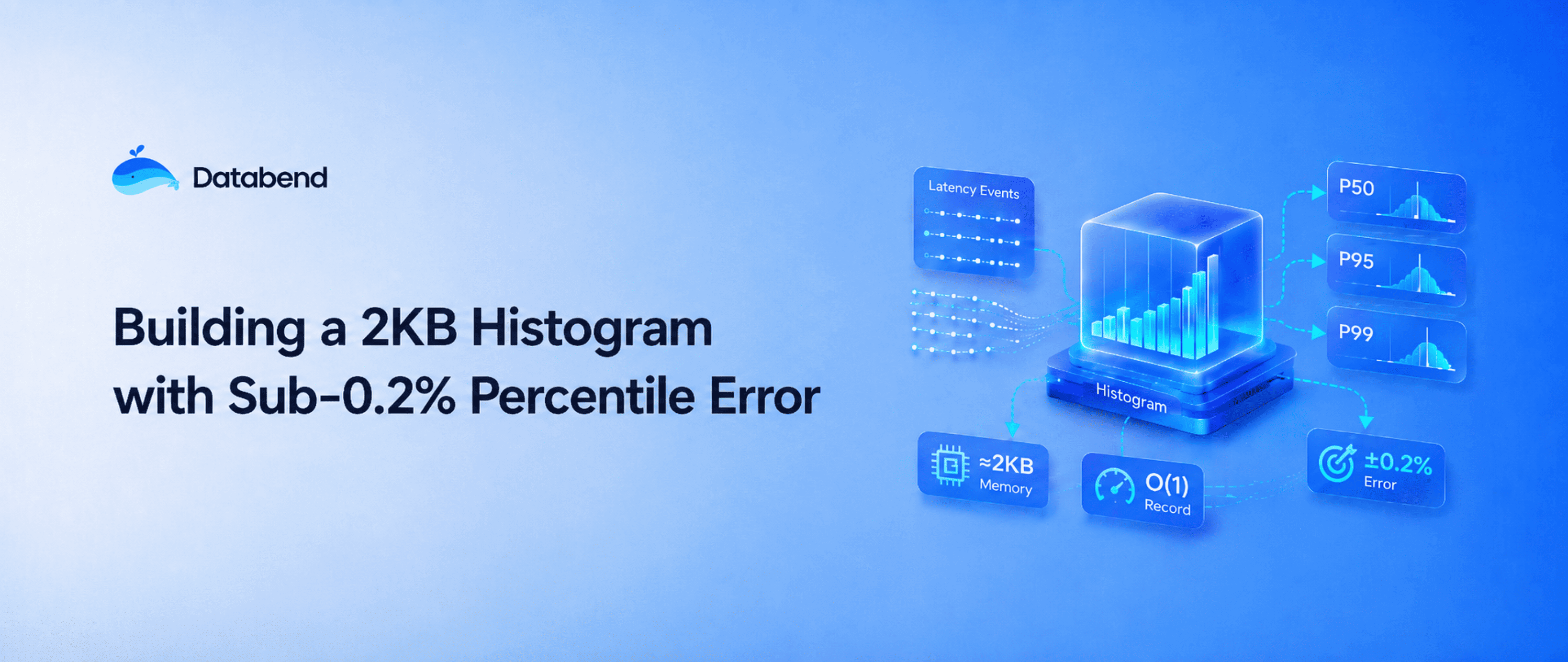
The Problem: Tracking Request Latency Without Slowing Things Down
For a cloud data warehouse, performance is not just about average query time. What often matters more is tail latency, predictability, and the ability to pinpoint where things go wrong.In a cloud-native data warehouse like Databend, a single request may pass through multiple stages: SQL planning, distributed execution, remote storage, Raft logging, and state machine apply. Tail latency in any one of these stages can affect the query stability users actually experience.
That means we need a way to continuously track latency distributions inside the system — lightweight enough to stay off the hot path, accurate enough to be useful, and cheap enough to run everywhere.
This article walks through the design of base2histogram, the lightweight histogram library we built for that purpose.
Consider the lifecycle of a single Raft log entry. It passes through several stages, each with its own latency profile:
-
Received → written to storage
-
Persisted to local disk
-
Replicated to remote nodes
-
Acknowledged by a majority quorum
-
Committed → applied to the state machine
A histogram is a natural fit here: put latency on the x-axis and request count on the y-axis, and you get an immediate view of where time is being spent.
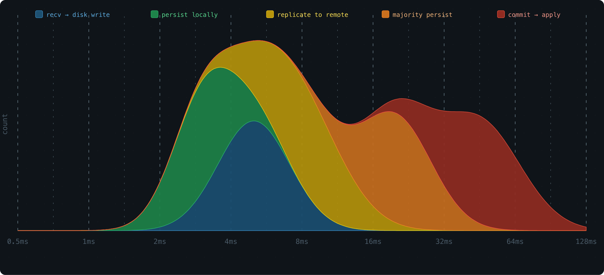
This kind of visibility helps you identify bottlenecks and fix the right part of the system.
But there is a catch: collecting metrics must not get in the way of doing actual work. The histogram needs to be:
-
O(1) to record — no sorting, no rebalancing, and nothing that can stall a hot path
-
Tiny in memory — a system may run hundreds or thousands of histograms at once
-
Queryable for percentiles — P50, P95, P99
Let's walk through how we designed a histogram that meets all three requirements.
Recording: Getting Samples Into Buckets
Why Log-Scale Buckets
Most requests cluster around a typical latency, with a few outliers on both ends. This often produces a log-normal distribution: take the log of the latency values, and the shape becomes a classic bell curve.
The signature shape is a peak at lower values, followed by a gradual long tail to the right.

To build a histogram, we divide the x-axis into buckets and count how many samples fall into each one.
The key question is how to size those buckets.
Equal-width buckets work well for a normal distribution, but latency is often log-normal. The data only looks roughly uniform on a logarithmic scale, so the buckets should grow on a log scale, not a linear one.
The simplest version is to make each bucket twice as wide as the previous one:
[0,1), [1,2), [2,4), [4,8), [8,16), ...
Why powers of 2? Because multiplying by 2 is cheap on a CPU, and mapping a value to its bucket takes a single leading zero count instruction.
If we simulate a log-normal workload and plot bucket counts with the bucket index on the x-axis — effectively applying a log transform — the result is a clean bell curve:
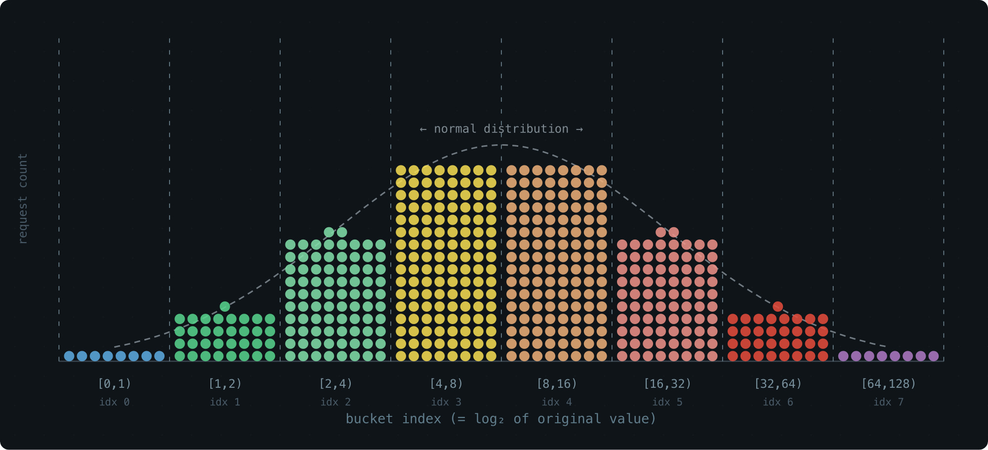
This is great for storage: 65 buckets cover the entire
u64
But the resolution is poor. The last bucket spans half of all possible values, so everything that lands there becomes a blur.
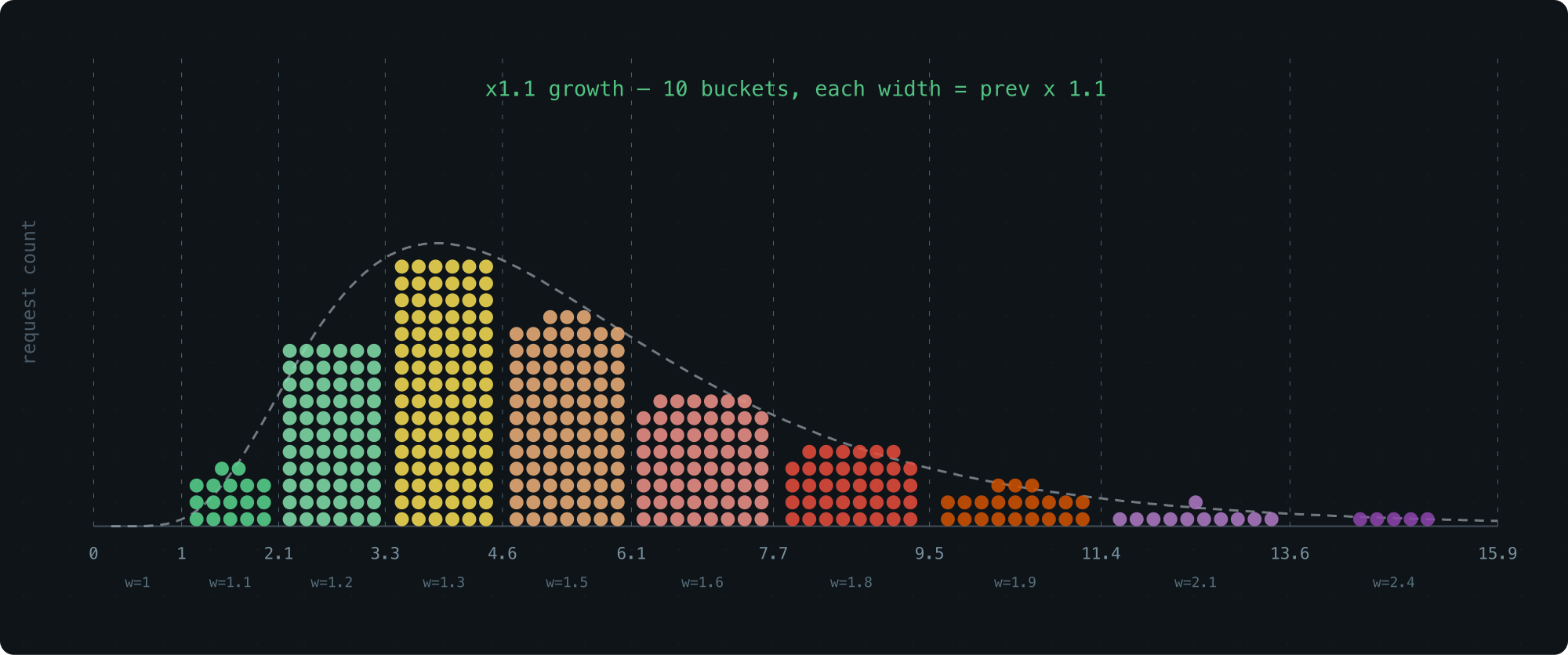
A Tempting Fix We Passed On
An obvious improvement is to use a smaller growth factor, such as 1.1× instead of 2×. That gives us more buckets and finer resolution:
The problem is cost. Finding the right bucket for a value
l
x
1 + 1.1 + 1.1^2 + ... + 1.1^x >= l
We wanted to stay in the world of integers and bit operations.
The Trick: Float-Like Encoding
Here is the idea that makes the design work: keep bucket sizes roughly exponential, but encode each bucket using a fixed number of bits — a parameter we call WIDTH.
Think of a bucket's lower bound as a tiny floating-point number.
The MSB position gives the exponent, which tells us which bucket group the value belongs to. The next few bits give the offset within that group.
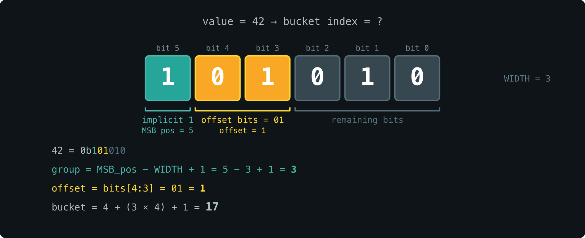
With WIDTH=3, the default configuration, a bucket boundary looks like this in binary:
00..00 1 xx 00..00
       |
       MSB
<- significant
The leading
1
Here is what the first few groups look like. Each bucket is fully described by just 3 bits:
WIDTH = 3:
range bucket index bucket size
[0, 1) 0 0b0 ..... 000 1
[1, 2) 1 0b0 ..... 001 1
[2, 3) 2 0b0 ..... 010 1
[3, 4) 3 0b0 ..... 011 1
[4, 5) 4 0b0 ..... 100 1
[5, 6) 5 0b0 ..... 101 1
[6, 7) 6 0b0 ..... 110 1
[7, 8) 7 0b0 ..... 111 1
[8, 10) 8 0b0 .... 1000 2
[10, 12) 9 0b0 .... 1010 2
[12, 14) 10 0b0 .... 1100 2
[14, 16) 11 0b0 .... 1110 2
[16, 20) 12 0b0 ... 10000 4
[20, 24) 13 0b0 ... 10100 4
[24, 28) 14 0b0 ... 11000 4
[28, 32) 15 0b0 ... 11100 4
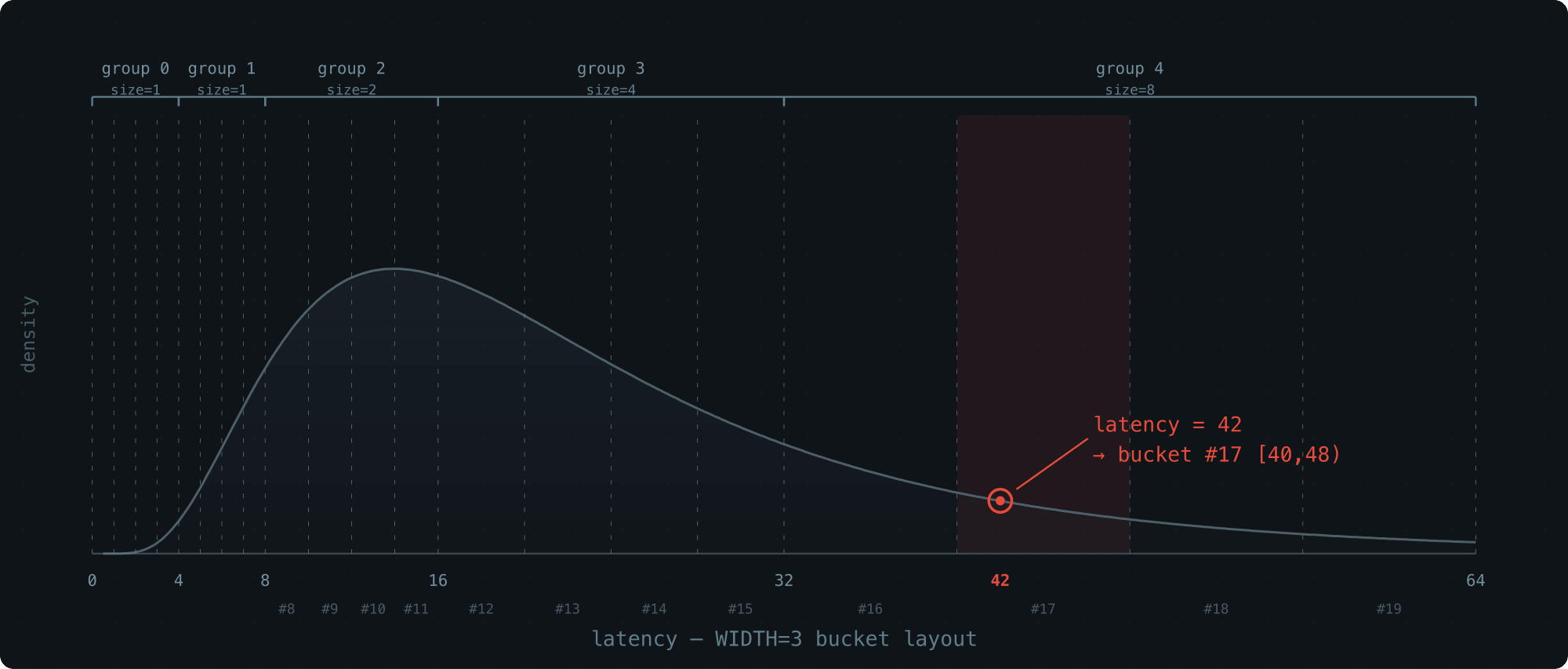
[32, 40) 16 0b0 .. 100000 8
[40, 48) 17 0b0 .. 101000 8
[48, 56) 18 0b0 .. 110000 8
[56, 64) 19 0b0 .. 111000 8
The pattern is simple:
-
Each group contains
buckets2^(WIDTH-1) = 4 -
The two bits after the MSB select the bucket within the group
-
It behaves like a 3-bit float: 1 implicit leading bit + 2 fractional bits
Bucket sizes still grow roughly logarithmically, but computing the bucket index is now just a matter of extracting the top WIDTH bits — a handful of integer and bit operations. Recording a sample is O(1).
Walk-through with latency = 42:
value = 42 (binary: 0b101010)
  MSB position: 5
  group: 5 - 2 = 3
  2 bits after MSB: 01 (from 1[01]010)
  offset in group: 1
  Bucket index: 4 + (3 × 4) + 1 = 17
Tuning WIDTH: The Precision–Memory Knob
WIDTH controls how many buckets each group contains:
2^(WIDTH-1)
The number of groups is capped at 64, so the histogram still covers the full
u64
Here is the trade-off:
| WIDTH | Buckets | Mem/slot | Buckets per group |
|---|---|---|---|
| 1 | 65 | 520 B | 1 |
| 2 | 128 | 1.0 KB | 2 |
| 3 | 252 | 2.0 KB | 4 (default) |
| 4 | 496 | 3.9 KB | 8 |
| 5 | 976 | 7.6 KB | 16 |
| 6 | 1920 | 15.0 KB | 32 |
At the default WIDTH=3, one histogram uses 2 KB and records every sample in O(1).
That covers the write path. Now let's look at the read path.
Percentile Estimation: Getting Answers Out
Once we have collected the counts, we want to query percentiles: at what latency have 50% of requests completed (P50)? What about 90% (P90) or 99% (P99)?
Locating the Right Bucket
The basic idea is simple.
For P50, count the total number of samples, take 50% to get a target rank
p
p
But a bucket spans a range, not a single point. We still need to estimate where inside the bucket the percentile falls.
Here are a few options, from rough to more accurate.
All error numbers below come from a log-normal distribution that models API latency, using WIDTH=3 and 1,000,000 samples.
Midpoint: return
(min + max) / 2
Many histogram libraries do this, including iopsystems/histogram. It is a blind guess: it ignores how samples are distributed within the bucket.
| P50 | P95 | P99 | |
|---|---|---|---|
| midpoint | 5.018% | 7.732% | 4.861% |
Uniform interpolation: assume samples are evenly spread across the bucket, then interpolate linearly:
estimate = min + (max - min) × rank / count
This is better than midpoint because it uses the target rank within the bucket. But the assumption is still rough: log-normal data is skewed, even inside a single bucket.
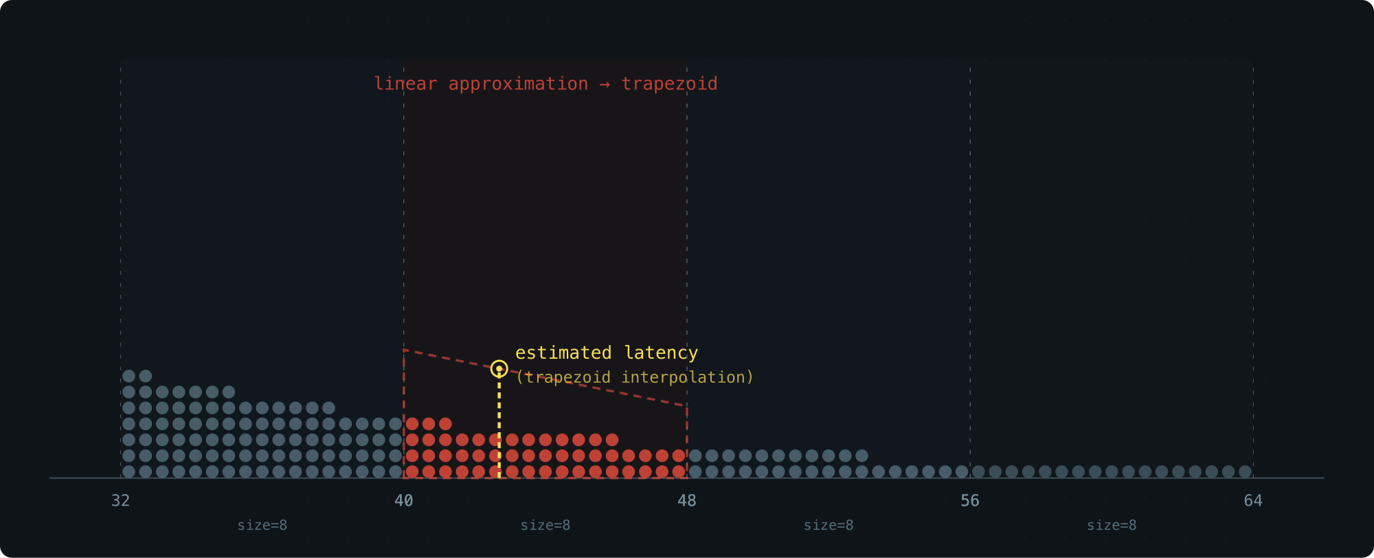
Trapezoid Interpolation (Our Approach)
Uniform interpolation treats density inside a bucket as flat. In reality, density is often sloped: higher on the side closer to the peak of the distribution.
If we can infer the direction and steepness of that slope, we can replace the rectangle with a trapezoid and get much closer to the true value.
Each bucket stores only a count, and we do not want to add any extra fields. So where does the slope information come from?
From the neighboring buckets.
The densities of the left and right buckets tell us how the density is likely to slope through the current bucket.
Here is the recipe.
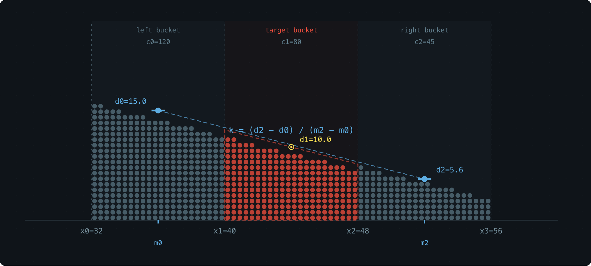
Compute the average density of the left bucket,
d0 = c0/(x1-x0)
m0
Do the same for the right bucket:
d2 = c2/(x3-x2)
m2
Then assume density changes linearly from
m0
m2
k
Inside the target bucket, the density now forms a trapezoid: a sloped line with slope
k
(x1+x2)/2
d1 = c1/(x2-x1)
To estimate the percentile, we solve for the x-position where the trapezoid area from
x1
Same distribution, same buckets — here is how the results compare:
| P50 | P95 | P99 | |
|---|---|---|---|
| midpoint | 5.018% | 7.732% | 4.861% |
| trapezoid | 0.000% | 0.080% | 0.086% |
That is two orders of magnitude better, with zero additional storage.
The three-bucket layout:
| Variable | Meaning |
|---|---|
| Boundaries of the three adjacent buckets |
| Bucket widths: |
| Sample counts in each bucket |
| How many samples into the target bucket the percentile falls |
d0 = c0 / w0       -- left bucket density
d1 = c1 / w1       -- target bucket density
d2 = c2 / w2       -- right bucket density
Midpoints of the left and right buckets:
m0 = (x0+x1)/2
m2 = (x2+x3)/2
Slope:
k = (d2 - d0) / (m2 - m0)
Then solve for the x-position where the trapezoid's cumulative area from
x1
The whole calculation uses only three counts and their bucket boundaries. Nothing else is stored, and nothing else is needed.
Benchmarks: Seven Distributions, Six WIDTH Settings
We tested the algorithm across seven representative distributions, each with 1,000,000 samples, using trapezoid interpolation.
The rows to focus on are LN-API and LN-DB at W=3. These are the real-world latency cases under the default 2 KB configuration:
|                   W=1      W=2      W=3      W=4      W=5      W=6
| ------------------------------------------------------------------
| Uniform P50    0.108%   0.028%   0.012%   0.018%   0.019%   0.002%
|         P95    2.317%   1.988%   1.035%   0.475%   0.005%   0.005%
|         P99    4.290%   4.129%   3.706%   1.486%   0.298%   0.162%
|
| LN-API  P50    2.281%   0.182%   0.000%   0.000%   0.000%   0.000%
|         P95   20.256%   3.963%   0.080%   0.040%   0.040%   0.000%
|         P99   11.951%   3.594%   0.086%   0.000%   0.029%   0.000%
|
| Bimodal P50    1.381%   0.394%   0.394%   0.197%   0.197%   0.197%
|         P95    3.918%   0.172%   0.012%   0.028%   0.038%   0.008%
|         P99    1.521%   1.344%   0.543%   0.078%   0.016%   0.014%
|
| Expon   P50    1.012%   0.000%   0.145%   0.145%   0.145%   0.000%
|         P95   10.989%   0.200%   0.000%   0.000%   0.033%   0.033%
|         P99   18.665%   4.574%   0.824%   0.022%   0.022%   0.022%
|
| LN-DB   P50    2.018%   0.034%   0.000%   0.000%   0.000%   0.034%
|         P95    2.027%   0.368%   0.039%   0.006%   0.019%   0.026%
|         P99    3.764%   1.066%   0.187%   0.007%   0.003%   0.062%
|
| Sequent P50    0.095%   0.000%   0.000%   0.000%   0.000%   0.000%
|         P95    2.271%   1.967%   1.011%   0.496%   0.000%   0.000%
|         P99    4.272%   4.118%   3.696%   1.521%   0.305%   0.169%
|
| Pareto  P50   10.127%   1.899%   0.633%   0.633%   0.633%   0.000%
|         P95    9.239%   0.272%   0.000%   0.136%   0.000%   0.000%
|         P99    3.517%   0.879%   0.231%   0.093%   0.046%   0.046%
|
| ------------------------------------------------------------------
| Buckets            65      128      252      496      976     1920
| Mem/slot        520 B   1.0 KB   2.0 KB   3.9 KB   7.6 KB  15.0 KB
| Mem total      1.0 KB   2.0 KB   3.9 KB   7.8 KB  15.2 KB  30.0 KB
What each distribution models:
-
Uniform (uniform distribution): synthetic benchmarks
-
LN-API (log-normal** σ=0.5)**: API and microservice latency
-
Bimodal (bimodal distribution): cache hit/miss — 90% fast path around 500 μs, 10% slow path around 50 ms
-
Expon (exponential distribution): network and I/O waits
-
LN-DB (log-normal σ=1.0): database query latency with a wider tail
-
Sequent (sequential): adversarial worst case
-
Pareto (Pareto distribution** α=1.5)**: heavy-tailed workloads, such as request sizes
For the latency distributions we care about most — LN-API and LN-DB — WIDTH=3 delivers sub -0.2% error with only 2 KB of memory.
Summary
-
2 KB memory: WIDTH=3, 252 buckets of
, with P50/P95/P99 error under 0.2% for log-normal latency workloadsu64 -
O(1) recording, O(buckets) querying
-
Trapezoid interpolation delivers over 10× better accuracy than midpoint, with zero extra storage
-
WIDTH is tunable: from 520 B for minimal tracking to 15 KB for maximum precision
A histogram may be a small piece of infrastructure, but it supports a much larger goal for Databend: making cloud data warehouse performance more observable, easier to reason about, and easier to optimize.
When a system can continuously record distributions such as P50, P95, and P99 at very low cost, engineering teams can trace tail latency much faster — whether it comes from storage, the network, Raft, the execution pipeline, or the query itself.
For users, that ultimately means more stable queries, more predictable performance, and a clearer path to cost optimization.
Check out the project: https://github.com/drmingdrmer/base2histogram
Subscribe to our newsletter
Stay informed on feature releases, product roadmap, support, and cloud offerings!