
From Traditional Partitions to Micro-Partitions—How Snowflake and Databend Reduce Data Scanning
 wubxAug 20, 2026

About This Series
A cluster key determines how records in a large table are physically grouped and, as a result, how much data a query must scan. Knowing the syntax is the easy part. Using a cluster key well requires answering three harder questions: why clustering works, how to choose an effective key, and how the implementation differs across platforms.
This series is designed to give data engineers a practical framework for deciding when clustering is useful, why it reduces scanning, whether the maintenance cost is justified, and how to verify that a design works.
The series currently includes two core articles, with a possible third installment:
-
Part 1—Concepts and mechanics (this article): Traditional partitions, Snowflake micro-partitions, Databend Fuse blocks, Min/Max pruning, range overlap, and the physical meaning of a cluster key.
-
Part 2—Design and operations: How to choose columns, order a composite key, select an appropriate time granularity, interpret clustering metrics, and manage automatic clustering or explicit reclustering.
Why Cluster Keys Start with Physical Data Placement
New users often interpret a Snowflake or Databend cluster key as an index, or as a persistent version of
ORDER BY
Why does better ordering reduce the amount of data scanned?
The answer lies in the full pruning path:
Write records into physical storage units
  -> Record column statistics for each unit
  -> Compare query predicates with those statistics
  -> Eliminate units that cannot contain a match
  -> Read only the remaining data
A cluster key improves the first step. By placing related values closer together, it makes the metadata created in the second step more selective and the pruning decision in the third step more effective.
As an initial mental model, think of a cluster key as an engine-maintained, dynamic form of range partitioning at the micro-partition or block level. This is useful intuition, but it does not make cluster keys equivalent to traditional hard partitions. We will return to that distinction later.
Snowflake and Databend support a similar high-level mental model built around fine-grained physical units, column statistics, pruning, and clustering. Their storage formats, background maintenance models, and operational interfaces are not identical.
Traditional Partitions: Users Define the Boundaries First
Consider a continuously growing table of LLM evaluation results:
CREATE TABLE llm_eval_results (
    created_at  TIMESTAMP,
    project_id  VARCHAR,
    eval_run_id VARCHAR,
    trace_id    VARCHAR,
    score       DOUBLE,
    passed      BOOLEAN
);
As evaluation jobs run, the table may grow to hundreds of millions or billions of rows. A traditional warehouse might define monthly range partitions:
2026-07 partition
2026-08 partition
2026-09 partition
On object storage, the same organization may appear as directory boundaries:
/year=2026/month=07/
/year=2026/month=08/
/year=2026/month=09/
Traditional partitioning has four defining properties:
-
The user chooses the partitioning column.
-
The user usually defines the boundaries in advance.
-
Each partition represents an explicit logical range.
-
A partition may still contain many files, row groups, or blocks.
For a one-day query:
WHERE created_at >= '2026-08-01'
  AND created_at <  '2026-08-02'
the engine can eliminate the July and September partitions and read only the August partition. This is traditional partition pruning.
The limitation is granularity. Partition pruning may narrow the search to one month, but the August partition can still contain a large amount of data. Without finer-grained metadata, the engine may need to read much of that partition. Coarse partitions therefore complement, rather than replace, pruning at the file, row-group, or block level.
Partition design also involves a familiar trade-off:
-
Boundaries that are too coarse leave too much data inside each partition.
-
Boundaries that are too fine create excessive metadata and small files.
-
New ranges may require ongoing boundary management.
-
A partition layout designed for one query pattern may become less useful when the workload changes.
Snowflake and Databend take a different approach to fine-grained organization. Users do not declare every small physical range. The engine forms storage units automatically according to data volume, write batches, and storage policy.
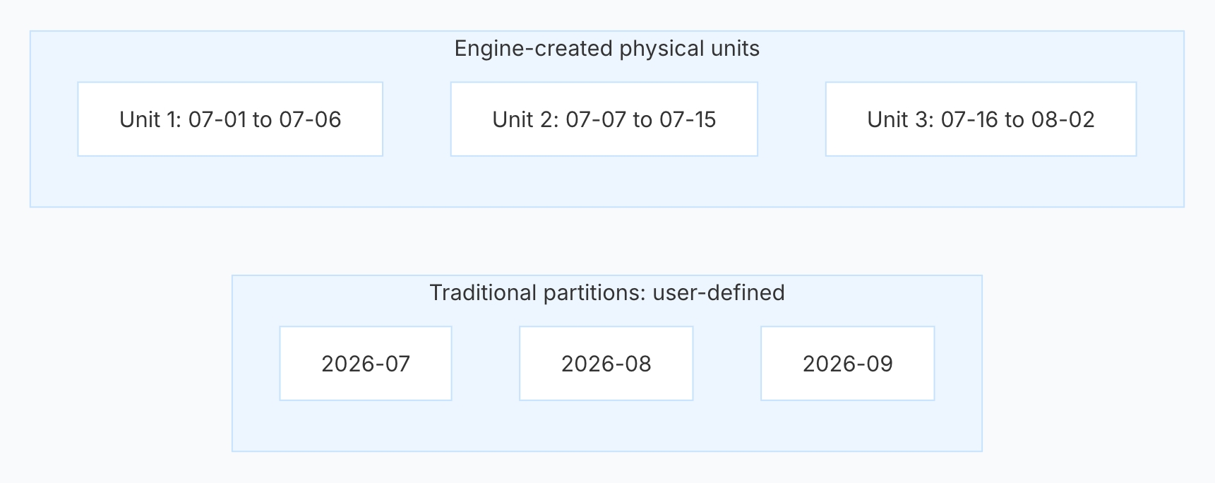
Figure 1. Traditional partitions use explicit, coarse boundaries. Engine-created micro-partitions or blocks are finer-grained and do not need to align with calendar months.
Micro-Partitions and Fuse Blocks: Units Created by the Engine
Snowflake automatically organizes table data into micro-partitions. Databend's Fuse engine writes data into blocks and groups multiple blocks into segments.
The implementations differ, but for the purpose of understanding cluster keys, both can be represented by the same simplified model:
Table
├── Physical Unit 1
├── Physical Unit 2
├── Physical Unit 3
└── Physical Unit 4
-
In Snowflake, a physical unit in this model is a micro-partition.
-
In Databend, it is a Fuse block.
The important distinction from traditional partitioning is who owns the boundary. Users do not normally define the range of each individual micro-partition or block. The engine creates these units and records metadata that can be used for pruning.
The most intuitive metadata is the minimum and maximum value of a column within each unit. Suppose the physical distribution of
created_at
Block A
created_at: [2026-07-01, 2026-07-07]

Block B
created_at: [2026-07-08, 2026-07-14]

Block C
created_at: [2026-08-01, 2026-08-07]
For the following predicate:
WHERE created_at >= '2026-07-10'
  AND created_at <  '2026-07-12'
the engine can compare the query interval with block metadata before reading column data:
-
Block A ends before July 10, so it can be skipped.
-
Block C begins after the query interval, so it can also be skipped.
-
Block B intersects the interval and must be read because it may contain matching rows.
This is Min/Max pruning, also commonly called data skipping.
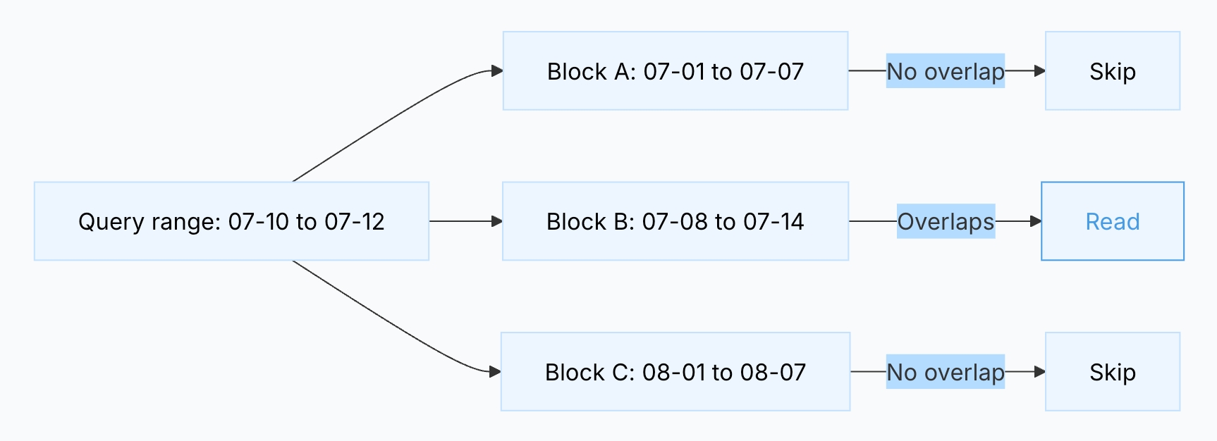
Figure 2. A physical unit can be skipped when its Min/Max range does not intersect the predicate. An intersection means only that the unit may contain a match.
That last point is an important limitation. Min/Max metadata can prove that a value is absent from a range, but it cannot prove that every value inside the range is present.
For example:
Block A trace_id: [trace_0001, trace_9999]
With this predicate:
WHERE trace_id = 'trace_5000'
the engine cannot eliminate the block using Min/Max metadata alone, even if
trace_5000
Databend can combine block-level Bloom filters with Min/Max pruning to eliminate more candidates for some equality predicates. Bloom filters and cluster keys solve different problems, however. A Bloom filter estimates whether a member may exist in a block; a cluster key changes the physical layout of the data itself.
Why Pruning Degrades: Wide and Overlapping Ranges
Min/Max pruning works best when values inside each physical unit are close together and ranges across units overlap as little as possible.
If data arrives in roughly chronological order, the layout may look like this:
Block A: [07-01, 07-07]
Block B: [07-08, 07-14]
Block C: [07-15, 07-21]
A query for July 10 needs only Block B.
Now consider concurrent ingestion combined with repeated historical backfills:
Block A: [07-01, 07-21]
Block B: [07-02, 07-20]
Block C: [07-03, 07-19]
The same July 10 query must retain all three blocks because each range may contain a match.
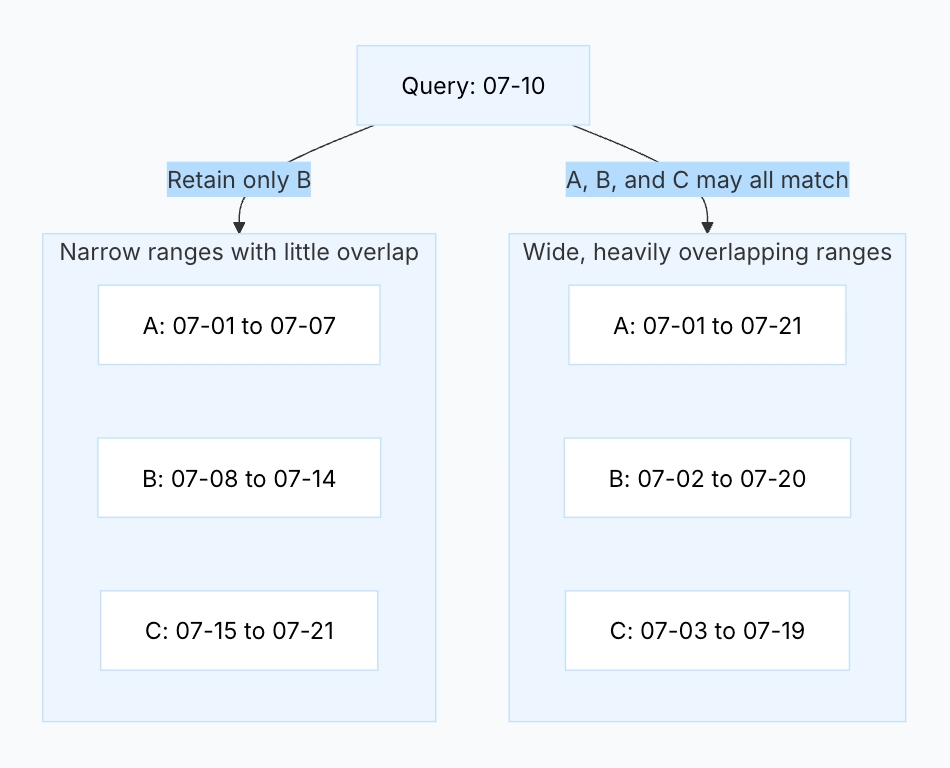
Figure 3. The same predicate can retain a completely different number of blocks depending on physical data layout.
Poor pruning does not necessarily mean the engine lacks statistics. More often, it means that:
-
each physical unit covers a wide value range;
-
ranges overlap heavily across units; or
-
the same key value appears in too many candidate ranges.
Overlap and clustering depth describe this condition. Intuitively, the more physical ranges that cover a given value, the more candidate units a query will usually retain. Snowflake exposes overlap and depth through functions such as
SYSTEM$CLUSTERING_INFORMATION
clustering_information
The central job of a cluster key is to reduce unnecessary range overlap.
What a Cluster Key Actually Changes
Suppose we define:
CLUSTER BY (created_at)
This does not create a traditional index on
created_at
Ideally, the layout evolves from wide, overlapping ranges:
Block A: [07-01, 07-21]
Block B: [07-02, 07-20]
Block C: [07-03, 07-19]
to narrower ranges with less overlap:
Block A: [07-01, 07-07]
Block B: [07-08, 07-14]
Block C: [07-15, 07-21]
The causal chain is straightforward:
Define a cluster key
  -> Bring similar key values closer together
  -> Narrow the value range of each physical unit
  -> Reduce overlap between physical units
  -> Allow Min/Max pruning to eliminate more candidates
  -> Scan less data
A cluster key is therefore not a direct lookup path. Unlike a B-tree, it does not resolve a predicate to a row identifier. Its benefit is indirect: it improves the physical layout so that existing pruning metadata becomes more selective.
Reclustering Maintains the Layout, but It Is Not Free
Continuous ingestion, updates, and historical backfills can gradually disrupt the layout. Reclustering selects some data and rewrites it into an organization closer to the cluster-key order.
That process consumes sorting, read, write, compute, and storage resources:
-
Snowflake primarily uses Automatic Clustering for background maintenance. Manual Reclustering is deprecated. The service consumes server-side resources and can incur credit and storage costs.
-
Databend also supports automatic clustering, while retaining explicit
control. Options such asALTER TABLE ... RECLUSTER,FINAL, andWHEREallow teams to control scope and depth. Explicit reclustering still consumes time and compute resources and incurs credits in Databend Cloud.LIMIT
The goal is not to make every micro-partition or block perfectly non-overlapping. A maintenance process should improve the most disordered ranges. Whether that work is worthwhile depends on whether the resulting reduction in query scanning exceeds the ongoing clustering cost.
Cluster Keys as Dynamic Range Partitioning
Traditional range partitioning follows this sequence:
User defines explicit ranges
  -> July 2026 goes to the July partition
  -> August 2026 goes to the August partition
  -> September 2026 goes to the September partition
Cluster-key-driven organization is different:
User declares the clustering dimension
  -> The engine forms physical units based on data volume
  -> Each unit derives Min/Max ranges from its actual contents
  -> Background maintenance adjusts the layout as data changes
After clustering by time, the resulting boundaries might look like this:
Block 1: [07-01 00:00, 07-03 15:20]
Block 2: [07-03 15:21, 07-08 09:10]
Block 3: [07-08 09:11, 07-19 18:40]
Block 4: [07-19 18:41, 08-02 11:30]
These boundaries are not encoded in the DDL. They emerge from the data distribution and target physical-unit size.
| Dimension | Traditional Range Partition | Cluster-Key-Driven Organization |
|---|---|---|
| Who defines the boundary? | The user defines it in advance | The engine derives it from the data |
| Typical granularity | Coarse business ranges | Micro-partition or block level |
| Is the boundary fixed? | Relatively stable | Changes with writes and clustering maintenance |
| What does the user declare? | Explicit partition ranges | Clustering columns or expressions |
| Primary value | Data management, lifecycle operations, and coarse pruning | Better physical locality and fine-grained pruning |
This comparison is useful because both approaches organize data by ranges. The boundary of the analogy is equally important:
A cluster key behaves like automatic, dynamic range partitioning at the micro-partition or block level, but it is not a traditional hard partition and does not guarantee that every physical unit fits inside a business-defined boundary.
Composite Keys: What (month, trace_id) Really Means
Column-selection strategy belongs in Part 2, but the physical meaning of a composite key is necessary to understand the mechanism.
If queries usually restrict a month before looking up a
trace_id
CLUSTER BY (
    DATE_TRUNC('month', created_at),
    trace_id
)
Interpret the tuple in lexicographic order:
Organize by month first
  -> Within the same or nearby month range, organize by trace_id
The resulting blocks may resemble:
Block 1: 2026-07 / trace_0001 ... trace_1000
Block 2: 2026-07 / trace_1001 ... trace_2000
Block 3: 2026-07 / trace_2001 ... 2026-08 / trace_0050
Block 4: 2026-08 / trace_0051 ... trace_1100
Block 5: 2026-08 / trace_1101 ... trace_2200
Block 3 can still cross the month boundary.
month
This layout is suited to queries that provide both constraints:
WHERE created_at >= '2026-08-01'
  AND created_at <  '2026-09-01'
  AND trace_id = 'trace_1024'
The engine can first eliminate physical units outside the month range, then use
trace_id
If the predicate contains only:
WHERE trace_id = 'trace_1024'
the same
trace_id
CLUSTER BY (month, trace_id)
trace_id
Part 2 will examine which columns should lead, whether time should remain at timestamp granularity or be reduced to day, week, or month, and when a high-cardinality identifier such as
trace_id
Snowflake and Databend: Shared Principle, Different Product Boundaries
Both Snowflake and Databend reduce scanning by combining automatically created physical units, column metadata, pruning, and clustered layouts. For users, the shared model is simple: improve physical locality so pruning can eliminate more data.
The operational experience is different.
| Dimension | Snowflake | Databend |
|---|---|---|
| Basic physical unit | Micro-partition | Fuse block; segments organize multiple blocks |
| Core role of a cluster key | Co-locate related records in more appropriate micro-partitions | Improve block-level physical organization using columns or expressions |
| Default maintenance model | Automatic Clustering evaluates and maintains the layout; Manual Reclustering is deprecated | Automatic clustering plus explicit |
| Explicit maintenance controls | Users can suspend or resume Automatic Clustering; resource management is primarily service-controlled | |
| Observability | System functions including | |
| Primary user model | Declare the clustering dimension, let the managed service maintain it, and monitor credit and storage impact | Declare the dimension, rely on automation when appropriate, and retain block-level observability and SQL-level intervention |
Snowflake: Managed Automatic Maintenance
Snowflake creates micro-partitions and maintains column metadata automatically. On very large tables where the natural ingestion order does not serve the dominant query path, users can define a clustering key and allow Automatic Clustering to evaluate and maintain the layout.
The product model is “declare the target and let the platform maintain it.” Users do not select a warehouse to execute reclustering, but they still need to account for the credits and storage impact of Automatic Clustering. A clustering key is not appropriate for every table. It is most relevant when a table contains many micro-partitions, queries are sufficiently selective, and access patterns are stable enough to benefit from one physical organization.
Databend: Automation with a Direct Physical Tuning Surface
Databend's Fuse engine organizes object-storage data into blocks and segments. After a cluster key is defined, the system can maintain the layout in the background. Databend also exposes the
RECLUSTER
clustering_information
This creates a two-layer operating model:
-
Declarative operation: Define the cluster key and allow the system to improve the layout continuously.
-
Observable intervention: Inspect block count, overlap, and depth, then explicitly control reclustering scope when operational requirements call for it.
The distinction is not simply “automatic versus manual.” It is a difference in product boundary. Snowflake emphasizes service-managed maintenance. Databend combines automatic clustering with a more direct SQL control plane. That control can help data teams align maintenance with batch windows or limit it to affected data ranges, but it also requires them to understand the compute, I/O, and write-amplification effects of explicit operations.
When a Cluster Key Is Worth the Cost
A cluster key should not be a default switch on every table in either platform. It is most likely to pay off when:
-
the table is large enough that queries scan many physical units;
-
important queries have stable, selective predicates;
-
the same clustering dimensions benefit a meaningful share of high-value queries; and
-
the cumulative query savings exceed the cost of initial reorganization and ongoing maintenance.
The incremental benefit is often limited when:
-
the table is small;
-
query predicates are highly variable or mostly unselective;
-
records naturally arrive in an order that already matches the main filters; or
-
writes and historical backfills disrupt the layout faster than clustering can economically maintain it.
Any physical layout favors some access paths over others. The relevant question is not whether a cluster key can make one query faster, but whether it reduces total scanning for the real workload at an acceptable maintenance cost.
The Mental Model to Keep
Partitioning, physical storage units, metadata, pruning, cluster keys, and reclustering form one continuous system:
Traditional partition
  -> User-defined, coarse-grained hard boundaries

Snowflake micro-partition / Databend Fuse block
  -> Fine-grained physical units created by the engine

Min/Max metadata
  -> Describes the value range that each unit may contain

Pruning
  -> Eliminates units that cannot satisfy a predicate

Cluster key
  -> Improves physical locality
  -> Narrows ranges and reduces overlap
  -> Allows pruning to skip more data

Reclustering
  -> Repairs the layout after continued writes
  -> Trades compute, I/O, and storage work for lower query scan cost
The important lesson is not a particular DDL statement. A cluster key is a physical-layout decision, not a SQL-syntax optimization. It improves one set of access paths and necessarily makes trade-offs against others.
The next article turns this model into a design process:
-
Which columns appear in stable, selective predicates?
-
How should columns in a composite cluster key be ordered?
-
Should a time field keep its original timestamp or be reduced to day, week, or month?
-
Are high-cardinality fields such as
andtrace_idsuitable cluster-key candidates?eval_run_id -
Why might low-cardinality fields such as Boolean or status columns provide little benefit?
-
Is clustering still necessary when the natural ingestion order is already close to the desired layout?
-
How should scan ratio, overlap, and depth be used to verify that a cluster key is effective?
These questions are covered in Cluster Key Series 02: Choosing Columns, Ordering Composite Keys, and Designing Granularity.
Subscribe to our newsletter
Stay informed on feature releases, product roadmap, support, and cloud offerings!